1.0 - Dynamic All-Pairs Shortest Paths Algorithms

• DIjkstra’s algorithm finds all shortest paths from one node
• The fastest implementation is $O(E=V\lg V)=O(V^2)$
• Running Dijkstra’s Algorithm from all nodes is therefore $O(V^3)$, however this cannot handle negative-weight edges.
• Bellman-Ford is $O(VE)=O(V^3)$ so with an extra loop for each nodes gives $O(V^4)$
• We can get $O(V^3)$ and handle negative-weight edges for all-pairs

1.1 - Recursive Definition of All-Pairs

• To solve this problem, we first define some notation

  • There are $N$ vertices, with IDs $1, 2, \cdots N$
  • Uses an adjacency-matrix representation, with $\text{weight}(i, j)$ as the weight of the edge from vertex $i$ to vertex $j$
  • If no edge exists, then the weight is $\infty$, hence return $\infty$ as the weight of the shortest path if one does not exist
  • $\text{weight}(v,v)=0, \forall v\in G.V$

• A path from vertex $i$ to $j$ can be either:

  • A path with no edges of weight $0$, e.g. $\langle i\rangle$ for $i=j$

  • A path with no more than one edge consisting of:

    • A path $p$, from vertex $i$ to some vertex $k$, and
    • The edge $\langle k, j\rangle$

    The weight of such path is $\text{weight}(p)+\text{weight}(k, j)$

• If the shortest path $\langle i, \cdots, k, j\rangle$ from $i$ to $j$ has $m$ edges, then

  • The path from $i$ to $k$ must have (at most) $m-1$ edges, and
  • It must be the shortest path from $i$ to $k$

• Let $\text{shortestPath}(i, j)^m$ repeat the weight of the shortest path from $i$ to $j$ with at most $m$ edges

  $$\text{shortestPath}(i, j)^0=\begin{cases}0&\text{if }i=j\\\infty&\text{otherwise}\end{cases}\\ \text{shortestPath}(i,j)^m=\min_{k\in V}(\text{shortestPath}(i, k)^{m-1}+\text{weight}(k, j))$$

  And hence, $\text{shortestPath}(i, j)^1=\text{weight}(i, j)$

• Since each sub-problem is described by 3 parameters, we require a 3d matrix to store the solutions

1.1.1 - Naive, Slow Solution

• We store $\textbf{shortestPath(i, j)}^m$ at $L[m, i, j]$ in an $n\times n\times n$ array $L$

• Calculate $L[1]$, then $L[2]$ from $L[1]$, then $L[3]$ from $L[2]$ etc

  slow_apsp(n)
      // L[m, i, j] is weight of the shortest path from i to j of at most m edges
      L = new int[n-1][n][n] // Initialise all elements to infinity.
      L[1] = weights
      for m = 2 to n - 1
          d = L[m-1]
          d' = L[m]
          for i = 1 to n
              for j = 1 to n
                  for k = 1 to n
                      d'[i, j] = min(d'[i, j], d[i, k] + weight(k, j))
  

• This algorithm is $T(n)\in \Theta(n^4)$ which is the same as running the Bellman ford algorithm $n$ times.

1.1.2 - Improved Solution

• We calculate $L[1]$ then $L[2]$, using $L[1]$
• Then $L[4]$ from $L[2]$
• Then $L[8]$ from $L[4]$

faster_apsp(n):
		// L[m, i, j] is the weight of the shortest path from i to j of at most m edges
    L = new int[2(n-1) - 1][n][n]
    L[1] = weights
    m = 1

    while m < n - 1
        d = L[m]
        d' = L[2m]
        for i = 1 to n
            for j = 1 to n
                for k = 1 to n
                    d'[i, j] = min(d'[i, j], d[i, k] + d[k, j])
        m = 2m

• Thus, this algorithm runs in $\Theta(n^3 \lg n)$ time

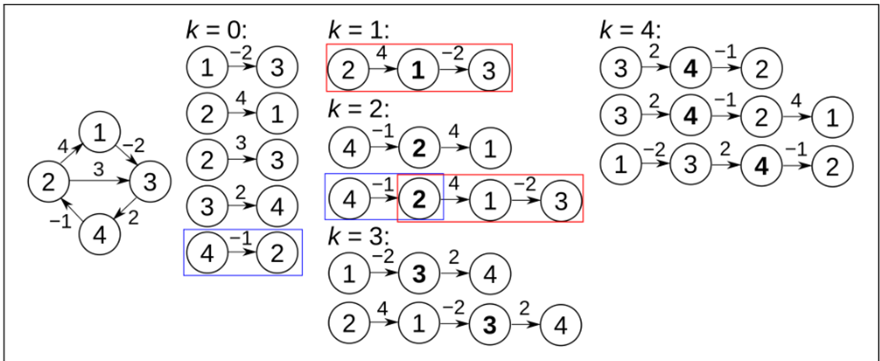
1.2 - Floyd Warshall Algorithm

• Why did we define our sub-problem in terms of path length?

• Instead, we can phrase our sub-problem in terms of which intermediate nodes are in the path

• Let $\color{lightblue}\text{shortestPath}(i, j, k)$ be the shortest path from $i$ to $j$, using only intermediate vertices $1\cdots k$

  • Remember that our vertices are conveniently ordered indices $1\cdots n$

• We incrementally add a new node to the intermediate set.

• Extending $1\cdots k$ to $1\cdots k+1$ requires checking whether the path formed by:

  • Going from $i\rightarrow k+1$ and $k+1\rightarrow j$ is better than already found.

• Let $\color{lightblue}\text{shortestPath}(i, j, k)$ be the weight of the shortest path from $i$ to $k$, using only intermediate vertices $1\cdots k$

  $\small\text{shortestPath}(i, j, k)=\text{weight}(i, j)\ \text{shortestPath}(i, j, k+1)=\min\begin{cases}\text{shortestPath}(i, j, k)\ \text{shortestPath}(i, k+1, k) + \text{shortestPath}(k+1, j, k)\end{cases}$

$\def\t{\ \ \ \ } 1\ \text{floyd-warshall}(W)\ 2\ \t n = W.\text{rows}\ 3\ \t D^{(0)} = W\ 4\ \t \bold{for\ } k = 1 \bold{\ to\ } n\ 5\ \t\t \text{let } D^{(k)}=(d^{(k)}{ij}) \text{ be a new } n \times n \text{ matrix}\ 6\ \t\t\bold{for\ } i = 1 \bold{\ to \ } n\ 7 \t\t\t \bold{for\ } j = 1\bold{\ to\ } n\ 8 \ \t\t\t\t d^{(k)}{ij}= \min(d^{k-1}{ij}, d^{k-1}{ik} + d^{k-1}_{kj})\ 9 \ \bold{return\ } D^{(n)}$

• This algorithm runs in $T(n)\in\Theta(n^3)$ time.

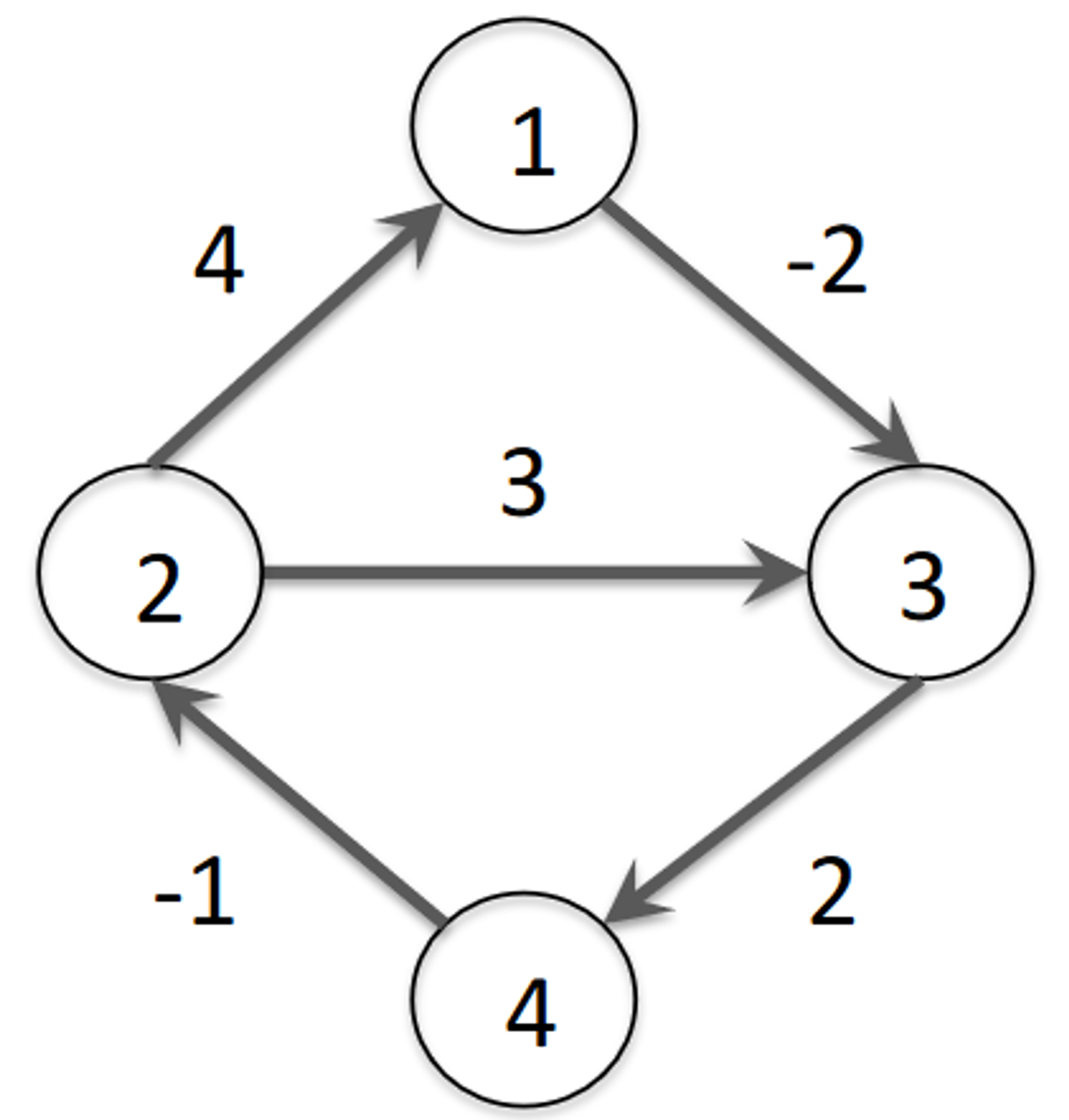
1.2.1 - Floyd Warshall Algorithm Example

1.3 - Aside: Johnson’s Algorithm

• Johnson’s Algorithm is $\Theta(V^3)$ in the worst case, but for sparse graphs is $\Theta(V^2 \lg V)$ using an adjacency list representation - in practice this isn’t always faster as it has very large constants associated with it.
• Our strategy is to
  1. Reweight to eliminate negative-weight edges
  2. Add a new source vertex.
     1. Run Dijkstra’s Algorithm for each node