Lindholm22 Chapter 2
A summary of Lindholm22 Chapter 2: Introduce the supervised machine learning problem as well as two basic Machine Learning methods for solving it.
- k-nearest neighbours
- decision trees
Supervised Machine Learning
- Given some training data that contains how examples of some input variable
relates to an output y, we want to use some mathematical model or method (which adapts / learns from the training data), we want to predict the output for some set of previously unseen test data, from which only is known.
Learning from Labelled Data
-
In most interesting supervised ML applications, the relationship between
and is difficult to describe explicitly. - Hard to express from application domain knowledge.
-
Therefore, cannot be solved by writing a computer program that takes
as an input and returns as output from a set of rules. -
Instead, learn the relationship between
and directly from the data, which contains examples of observed pairs of input and output values. - Supervised Machine Learning amounts to learning from examples
-
The data used for learning is called training data, and consists of several input-output data points
. -
We will compactly represent the training data as
for training data with pairs. -
Each data point in the training data provides a snapshot of how
depends on - The goal is to squeeze as much information as possible about
- The goal is to squeeze as much information as possible about
-
The fact that the training value doesn't only contain input values, (but also output values / labels) is the reason for the term
supervised machine learning.- We may say that each input
is accompanied by a label , or simply that we have labelled data
- We may say that each input
-
For some applications, it is only a matter of recording
and . - However, for other applications, the output
has to be created by labelling of the training data inputs by a domain expert.
- However, for other applications, the output
-
Note that the vector boldface notation
is used to denote the input, since we assume it is a -dimensional vector, (where ) denotes the transpose of the matrix.
x=\begin{bmatrix}x_1&x_2&\cdots &x_p\end{bmatrix}^T \tag{1}
-
Each element of the vector input
represents some information that is considered to be relevant for the application at hand, for the application at hand. - In many applications, the number of inputs
is large.
- In many applications, the number of inputs
-
For instance, in a computer vision application, where the input is a greyscale image,
can be all pixel values in the image, so where and denote the height and width of the input image. -
The output
, on the other hand, is often low dimension, and throughout most of this book, we will assume that it is a scalar value. -
The type of the output value, numerical or categorical, turns out to be important and is used to distinguish between two subtypes of the supervised machine learning problems: regression and classification.
Numerical and Categorical Variables
-
The variables contained in our data can be of two different types: numerical or categorical.
- A
numerical variablehas a natural ordering.- One instance of a numerical variable is larger than (or smaller than) another instance of the same variable.
- Could be discrete or continuous
- A
Categoricalvariable is always discrete and lack natural ordering- Assume that any categorical variable can take a finite number of values.
- A
-
Sometimes there is some ambiguity as to whether an output is a categorical or numerical variable - up to the decision of the ML Engineer.
-
This notion of a variable being categorical or numerical applies to both the output variable
and the input variable shown in equation (2) below.
\bf{x}=\begin{bmatrix}x_1&x_2&\cdots&x_p\end{bmatrix}^T \tag{2}
- Note that the
input variables don't have to be of the same type.
Classification and Regression
Regression: Output is numericalClassification: Output is categorical
-
Distinguish between different supervised ML problems by the type of the output of
. -
This distinction must be made as classification and regression problems have somewhat different properties, and thus different methods are used to solve them.
-
Note that the
input variables in Eq (3) below can either be numerical or categorical (or a mix of both) for both classification and regression problems.
\bf{x}=\begin{bmatrix}x_1&x_2&\cdots&x_p\end{bmatrix}^T \tag{3}
-
It is only the type of the output that determines whether a problem is a classification or regression problem.
-
A method for solving classification problems is called a
classifier.- For classification, the output is categorical and can therefore only take values in a finite set.
- We use
to denote the number of elements in the set of output values as shown in the table below.
| Possible Output Values | M |
|---|---|
| 2 | |
| 4 |
- We refer to these elements as classes or labels.
- The number of classes
is assumed to be known for the classification problem.
- The number of classes
- Use the integers
to denote the output classes for . - The ordering (mapping of class # to class name) is arbitrary and does not imply any ordering of the classes.
- When there are only 2 classes, we have the important special case of
Binary Classificationand thus we use the label set. - We will occasionally use the equivalent terms positive and negative class.
- Only reason for this change is that it gives a more compact mathematical representation for some methods.
Example - Classifying Songs
- Want to classify whether song has artistic style of
- Require mechanism that goes from audio recording -> artist's name
- Collect dataset of songs and respective labels (artists' names).
- learn characteristics of different styles and therefore predict the artists of the song provided from the user.
- Need to consider what input
really is - In principle, able to consider the raw audio format as the input, but would give very high-dimensional shape of
. - Unless using audio-based learning model, dimensionality is probably too high and unrealistic amount of training data to train.
- Can instead consider some summary statistics of audio recordings, and use those features as input
instead. - These features could include the length and the perceived energy of the song.
- The derivation of the perceived energy of the song is difficult to quantify, but we assume that a piece of software takes in the song, and deterministically returns a number representing the song.
- In principle, able to consider the raw audio format as the input, but would give very high-dimensional shape of
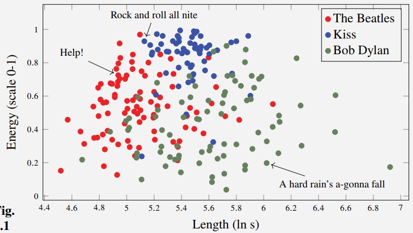
Note With many machine learning tasks, it is not reasonable to get 100% accuracy - looking at the scatter plot, there aren't enough good features to separate the song classes. We could achieve higher accuracy (greater separation between classes) with more features, or better features.
Generalising Beyond Training Data
Two reasons why it can be of interest to mathematically model the input-output relationships from training data.
- To reason about and explore how input and output variables related. e.g. is there correlation between a pair of variables.
- To predict the output value
for some new, previously unseen input . Using some mathematical method that generalises the input-output examples seen in the training data, we can make a prediction for some previously unseen . Note here that the hat symbol denotes that the prediction is an estimate of the output.
k-Nearest Neighbours
-
We can use the
-nearest neighbours ( -NN) method, which can be used for regression and classification. -
Remember that we have access to training data, denoted
consisting of data-points, with input vector and corresponding output . -
From this training data, we want to construct a prediction
for what we believe the output would be for some new , which we have not previously seen. -
Most methods for supervised Machine Learning build on the intuition that if the test data point
is close to the training data point then the prediction should be close to . -
One simple way to implement this in practice is:
- Compute the euclidean distance between the test input and all training inputs as shown in Eq. (4) below
||\bf{x}_ i-\bf{x_ \star}||\ \forall i\in\lbrace 1,\cdots,n\rbrace\tag{4}
- Find data point
in the training set with the shortest distance to and use it's output as the prediction:
\hat{y}(\bf{x_\star})=y_j \tag{5}
- This simple prediction method is known as the 1-nearest neighbour method.
- Not very complicated, but for most machine learning applications it is too simplistic and the data is often noisy (affected by random errors.)
- To improve the 1-nearest neighbour method, we can extend it to make use of the
-nearest neighbours instead. - Formally, we define the set:
\mathcal{N}_ \star=\{i: \bf{x_ \star \text{ one of the }k\text{ training data points closest to } \bf{x_ \star}}\} \tag{6}
- For regression problems, we take the average of all
. - For classification problems we use a majority vote.
Note: We don't care about the model's performance on the dataset used for training - we want to evaluate the model on data it hasn't seen before (testing the model's ability to generalise).
- Methods that explicitly use the training data when making predictions are referred to as non-parametric, and the
-NN method is one example of this. - This is in contract to parametric methods, where the prediction is given by some function (a model) governed by a fixed number of parameters.
- For parametric methods, the training data is used to learn parameters in an initial training phase, but once the model has been learned, the training data can be discarded since it is not used explicitly when making predictions.
The
Data: Training data, denoted
Result: Predicted test output,
- Compute the distances
for all training points - Let
- Compute the prediction
using the following formula:
\hat{y}(\bf{x_ \star})=\begin{cases}\text{Average}\{y_ j:j\in\mathcal{N}_ \star\}&\text{(Regression problems)}\\ \text{MajorityVote} \lbrace y_ j : j \in \mathcal{N}_ \star\rbrace &\text{(Classification problems)}\end{cases}\tag{7}
Example - Predicting Colours with
- Consider a synthetic binary classification problem (
). We are giving a training dataset with observation of input variables, , and one categorical output , the color or .
| 1 | -1 | 3 | |
| 2 | 2 | 1 | |
| 3 | -2 | 2 | |
| 4 | -1 | 2 | |
| 5 | -1 | 0 | |
| 6 | 1 | 1 |
- We are interested in predicting the output for
\bf{x_\star}=\begin{bmatrix}1&2\end{bmatrix} \tag{8}
-
Explore two different
-NN classifiers, and $k=3 below: -
The first step is to compute the Euclidean distance
between each training point . and the test data point and then sort them in ascending order.
| 6 | ||
| 2 | ||
| 4 | ||
| 1 | ||
| 5 | ||
| 3 |
- We can then generate the following plot of our points, observing that:
- The black dot is the point that we want to try to infer the class (color) of
- When
there only dot is considered when predicting the class label of the black dot. - When
dots are considered when predicting the class label - Since there are 2 blue dots and 1 red dot, the class of the black dot is
via majority vote.
- Since there are 2 blue dots and 1 red dot, the class of the black dot is

-
In the above example, we only compute the prediction for a single test data point,
. -
Whilst this may be the ultimate goal of our model, to better understand the classifier, we want to study it's decision boundary.
-
It is a general concept for all types of classifiers, but can only really be easily visualised with classifiers when the dimension of
is . -
We can sweep through a range of values in the variable space, and determine where the boundaries of each classification were:
- Sweep through each point, and predict using the
-NN model the class for that particular point. - Precisely at this decision boundary, the classification is undetermined, and can be determined by a coin flip.
- However, this is highly unlikely that a data-point will like exactly on the decision boundary.
- Sweep through each point, and predict using the
-
For all classifiers, end up with points in the input space where the class prediction abruptly changes from one class to another.

Choosing k
- The number of neighbours considered when making a prediction using a
-NN is an important choice that the user must make. - Since
is not learned by the model itself (it is a design choice left to the user), we refer to it as a hyperparameter. - Refers to tuning parameters that must be set by the user.
- The choice of the hyperparameter
has a big impact on the predictions made by the -NN as seen in the example above. - With
, all training data-points will be correctly predicted, and the model is adapted to the exact and values of the training data. - The drawbacks of using
is that most real-world problems have an element of randomness in the data (or at least, insufficient information which can be thought of as a random effect). - If we want our classifier to be able to generalise to completely new data, then it would not be reasonable that this insufficient information is able to give a complete picture of the data.
- The drawbacks of using
- We want to choose a value of
such that we are adapting very closely to the training data, but we are not fitting to the random effects on the training data (i.e. over-fitting).
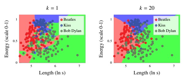
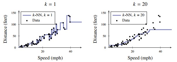
- With
-NNs, we can mitigate over-fitting by increasing the region of the neighbourhood used to compute the prediction (increase ). - With
, the predictions are no longer based on the closest neighbour, so not all training points are perfectly classified so some end up in the incorrect region - Predictions are less adapted to the peculiarities of the training data, and thereby less over-fitted.
- However, if
is too large, then the averaging effect will wash out all the interesting patterns of the data. - Therefore, setting
is a trade-off between flexibility and rigidity. - No general answer, depends on the problem
Input Normalisation
- Imagine a training dataset with
input variables, where all values of are in the range and the values for are in range . It could be, for example that are measured in different units. - The Euclidean distance between a test point
and a training data point is given by:
||\bf{x_i}-\bf{x_\star}||_2=\sqrt{(x_{i1}-x_{\star 1})^2 + (x_{i2}-x_{\star 2})^2}.
-
This expression will typically be dominated by the first term
whereas the second term tends to have a much smaller effect, simply due to the different magnitude of and . -
Different ranges lead to
being considered much more important than by the -NN -
To avoid this undesired effect, we can re-scale the input variables. One option, in the mentioned example, could be to subtract 100 from
and thereafter divide it by and create such that and are both in the range . -
More generally, this normalisation procedure for the input data can be written as:
x_{ij}^{\text{new}}=\frac{x_{ij}-\min_{\ell}(x_{\ell j})}{\max_\ell (x_{\ell j})-\min_\ell(x_{\ell j})},\ \ \ \ \ \ \ \ \forall j\in\lbrace 1, \cdots, p\rbrace,\ \ i\in \lbrace 1, \cdots, n\rbrace
- Another common normalisation approach (standardising) is by using the mean and standard deviation in training data:
x_{ij}^{\text{new}} = \frac{x_{ij}-\bar{x}_j}{\sigma_j}, \ \ \ \ \ \ \ \ \forall j\in\lbrace 1, \cdots, p \rbrace, \ \ i \in \lbrace 1, \cdots, n \rbrace
Decision Trees
- The
-NN method results in a prediction that is a piecewise constant function of the input . - Partitions the input space into disjoint regions, and each region is associated with a certain (constant) prediction.
- For
-NN, regions are implicitly defined by the -neighbourhood for each possible test input - An alternative approach is to devise a set of rules that defines the regions explicitly.

- Consider the music data from before, in which a simple set of high-level rules for constructing a classifier could be:
- Inputs to the right are classified as Green (Bob Dylan)
- Inputs to the left are classified as Red (The Beatles)
- Inputs to the top are classified as Blue (Kiss).
- We can learn these rules systematically from training data.
Example - Predicting Colours with a Decision Tree
- Consider a classification problem with two numerical input variables
and one categorical output with values . - How can we use (an existing) decision tree to predict
?
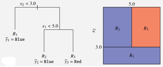
- The rules defining the model are organised in the decision tree in the left of Figure 3.
- To use this tree to predict a label for the test input
, we start at the top (root node) of the tree. - If the condition proposed is true, we traverse the the left branch of the tree, otherwise we traverse the right branch of the tree.
- Upon reaching a new internal node of the tree, we evaluate the condition, and traverse the left branch (if condition is true) or right branch.
- We continue to work our way down until we reach the end of a branch (leaf node), each of which correspond to a constant prediction
- To use this tree to predict a label for the test input
- The decision tree partitions the input space into axis-aligned boxes as shown in the right of Figure 3.
- By increasing the depth of the tree (# of steps from root
leaves), the partitioning can be made finer and finer (thereby describing more complication functions of the input variable(s)).
function predict(x_1, x_2):
  if x_2 < 3.0:
    return Blue
  else:
    if x_1 < 5.0:
      return Blue
    else:
      return Red
- For example, if we have
, in the first split, we would take the right branch since and in the second split, we would take the left branch since . The prediction for this test point would be
- With more than two input variables, it is difficult to illustrate the partitioning of the input space into regions, but the tree representation can still be used in the same way. Each internal node corresponds to a rule where one of the
input variables is compared to some threshold . - If
we continue along the left branch, and if then we continue along the right branch.
- If
- The constant predictions associated with leaf nodes can be categorical or numerical - decision trees can be used for both classification and regression problems.
Learning a Regression Tree
- The prediction
from a regression tree is a piecewise constant function on the input . We can write this mathematically as:
\hat{y}(\bf{x_\star})=\sum_{\ell=1}^{L} \hat{y}_\ell \mathbb{I}\lbrace \bf{x}_\star \in R_\ell \rbrace
-
Total number of regions (leaf nodes) in the tree -
is the th region. -
is used as the indicator function where: if if
-
Learning the tree from data corresponds to finding suitable values for the parameters defining the above functions, namely the regions
and the constant predictions as well as the total size of the tree, . -
If we start by assuming that the shape of the tree, the partition
is known, then we can compute the constants as the average of training points in each region
\hat{y}_\ell=\text{Average}\lbrace y_i : \bf{x}_i \in R_\ell\rbrace
- We still need to find the shape of the tree, the regions
- Want to select regions such that the tree fits the training data
- Output predictions from the tree should match the outputs in the training data.
- Finding a tree that optimally partitions the input space to fit the training data as well as possible turns out to be computationally infeasible - combinatorial explosion in number of ways tp partition space.
- To get around this, we can use a heuristic algorithm known as recursive binary splitting for learning the tree.
- Start with the first split at the root, building the tree from top to bottom
- An example of a greedy algorithm, constructed one split in tree.
- Consider when we are about to do the very first split at the root of the tree
- Want to select one of the
input variables, and a corresponding cut point that divides the input spaces into two half-spaces:
- Want to select one of the
R_1(j,s)=\{\bf{x} | x_j < s\}\ \ \ \ \ \ \ \
\text{and}
\ \ \ \ \ \ \ \ \ R_2(j,s)=\{\bf{x} | x_j \ge s\}\tag{2.4}
- Note that the regions depends on the index
of the splitting variable, as well as the value of the cut-point , which is why we write them as functions of and . This is the case for predictions associated with the two regions, in which the averages depend on the different data-points within their respective regions.
\hat{y}_1(j,s)=\text{Average}\{y_i:\bf{x}_i\in R(j,s)\}
\ \ \ \ \ \ \ \ \ \ \ \text{and}
\ \ \ \ \ \ \ \ \ \ \ \hat{y}_2(j,s)=\text{Average}\{y_i : \bf{x}_i \in R_2(j,s)\}
- For each training data-point
, we can compute a prediction error, by first determining which region the data-point falls in, and then computing the difference between and the constant prediction associated with that region. Doing this for all training data-points, the sum of squared errors can be written as:
\sum_{i: \bf{x}_i\in R_1(j,s)} (y_i-\hat{y}_1(j,s))^2 + \sum_{i: \bf{x}_i\in R_2(j,s)} (y_i-\hat{y}_2(j,s))^2\tag{2.5}
- The square is added to ensure that the expression above is non-negative, and that both positive and negative errors are counted equally.
- The squared error is a common loss function used for measuring the closeness of a prediction to the training data, but other loss functions can also be used.
Finding the Optimal Split
- Want to select the values for
and that minimise the squared error. - This minimisation problem can be solved easily by looping through all possible values for
. - For each
, scan through all possible splits and pick the pair for which the above expression is minimised. - Continue for left and right branches independently, minimising the squared prediction error along the way.
- For each
- Conceptually, can continue until there's only a single training point in each of the regions
. - Similar to
-NN with .
- Similar to
- This typically results in an erratic model that has over-fitted to the training data.
- Common to stop the growth of the tree at an earlier stage using some stopping criterion (e.g. by deciding
beforehand.) or adding a constraint on the minimum number of training data points associated with each leaf node - Constraining # of training points in leaf node results in an averaging effect, similar to
for -NN.
- Constraining # of training points in leaf node results in an averaging effect, similar to
Classification Trees
- Can use trees for classification.
- Modify the binary splitting algorithm from before, with two major differences:
- Use majority vote instead of average to compute the prediction associated with each region
- When learning the tree when the output is categorical, we need to define a different splitting criterion than the squared prediction error to take into the fact that the output is categorical.
- To define this, note that the split at any internal node is computed by solving the optimisation problem of the form:
Number of training points in the left and right nodes of the training split costs (derived from prediction errors) associated with the two nodes. Variables that denote the index of the splitting variable, and the cut-point (as before) - Note that this is the same equation as Eq 2.5 if
corresponds to the mean-squared error in node
Generalisation to Classification Case
- We still solve the optimisation problem in Eq 2.6 to compute the split, but choose
in a different way.
\hat{\pi}_{\ell m}=\frac{1}{n_\ell} \sum_{i : \bf{x}_i\in R_\ell} \mathbb{I}\{y_i=m\}
- Let the above formula denote the proportion of training observations in the
th region that belong to the th class. - We can then define the splitting criterion
based on the class proportions.
- We can then define the splitting criterion
- One simple alternative is the misclassification rate which is the proportion of data-points in the region
which do not belong to the most common class.
Q_\ell=1-\max_{m} \hat{\pi}_{\ell m} \tag{2.7a}
- Another common splitting criteria is the Gini index
Q_\ell =\sum_{m=1}^M \hat{\pi}_{\ell m} (1-\hat{\pi}_{\ell m}) \tag{2.7b}
- Finally, we have the entropy criterion
Q_\ell=-\sum_{m=1}^M \hat{\pi}_{\ell m} \ln \hat{\pi}_{\ell m} \tag{2.7c}
- When choosing between different splitting criteria, misclassification rate sounds like a reasonable choice, since that is typically how we evaluate a model's performance
- However, it doesn't favour pure nodes (regions where most of the data-points belongs to a certain class)
- Usually favourable to favour pure node in the greedy procedure used to grow the tree, since this can lead to fewer splits in total.
- Both the entropy criterion and Gini index favour node purity more than the misclassification rate.
Learning a Decision Tree
Goal: Learn a decision tree using recursive binary splitting:
Data: Training data Result: Decision tree with regions
- Let
denote the whole input space - Compute the regions
- Compute the predictions
for as: \hat{y}_\ell=\begin{cases} \text{Average}\{y_i:\bf{x}_i \in R \ell\} & \text{(Regression Problems)}\\ \text{MajorityVote}\{y_i : \bf{x}_i\in R\ell \} &\text{(Classification Problems)}\\ \end{cases}
Function Split(R, 𝒯):
    if (stopping criterion fulfilled)
        return r
    else
        Go through all possible splits xⱼ < s for all input variables
          j = 1, ..., p
        Pick the pair (j,s) that minimises the loss function for regression/classification problems
        Split the region R into R₁ and R₂ according to Eq 2.4
        Split data 𝒯 into 𝒯₁ and 𝒯₂ respectively
        return Split(R₁, 𝒯₁), Split(R₂, 𝒯₂)
Predicting from a Decision Tree
Data:
- Decision tree with regions
- Training data
- Test data point
Result: Predicted test output
- Find the region
to which belongs. - Return the prediction
Example - Learning a Classification Tree
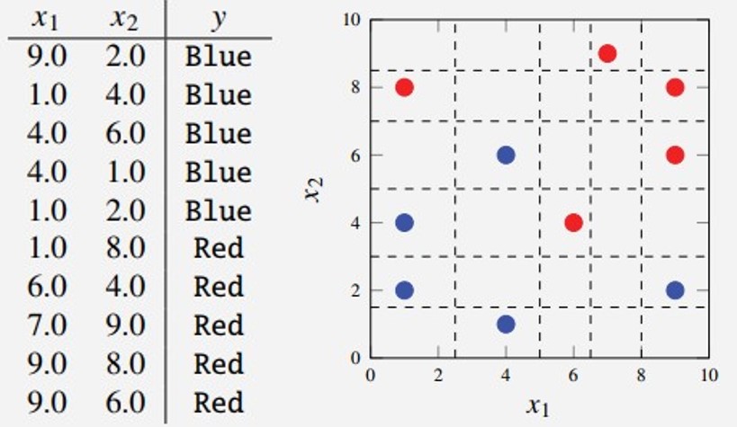
- Consider the above data, for which we want to learn a classification tree.
- First Split There are infinitely many possible splits that we can make, but all splits which give the same partition of the data-points are equivalent.
- Hence, in practice, we only have nine different splits to consider in the dataset
- The data (dots) and these possible splits (dashed lines) are visualised in the figure above.
- Consider all splits in turn - begin with split at
which splits the input space into two regions:
R_1=x_1<2.5, R_2=x_1\ge 2.5
- In region
we have two blue data-points and one red = . - Therefore, the proportion of the two classes in region
will therefore be and - Then, the entropy is calculated as:
- Therefore, the proportion of the two classes in region
Q_1= -\hat{\pi}_{1B} \ln(\hat{\pi}_{1B})-\hat{\pi}_{1R} \ln(\hat{\pi}_{1R})=-\frac{2}{3}\ln(\frac{2}{3})-\frac{1}{3}\ln(\frac{1}{3})=0.64
- In region
, we have data points with
Q_2= -\hat{\pi}_{2B} \ln(\hat{\pi}_{2B})-\hat{\pi}_{2R} \ln(\hat{\pi}_{2R})=-\frac{3}{7}\ln(\frac{3}{7})-\frac{4}{7}\ln(\frac{4}{7})=0.68
- Inserting these two figures into Eq (2.6), the total weighted entropy for this split becomes:
n_1 Q_1 + n_2 Q_2 = 3\cdot 0.64 + 7 \cdot 0.68 = 6.69
- We can continue computing these costs for all other splits in the same manner, and summarise them in the table below:
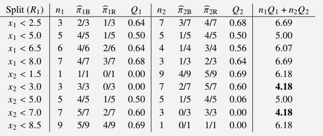
- From the table, we can read that the two splits at
and are both equally good. - We choose to continue with
- Second Split We note that only the upper region has more than give data-points. Also, there is no point splitting
further, given it only contains data-points from a single class. - We therefore split the upper region into two new regions,
. - All possible splits are displayed below (left) and we compute the costs in the same manner as before:
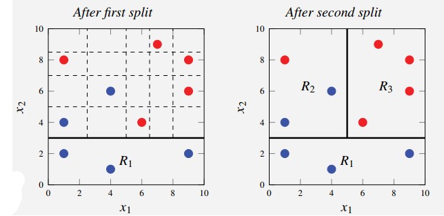

- The best split is the one at
, shown to the right of the above picture. None of the three regions have more than give data-points, and thus we terminate the training. - The final tree and its partitions are shown in Example 2.5 above.
- Using the tree for prediction, we predict
if or since the blue training data points are in the majority in each of these two regions - Similarly, if
we predict