COMP4702 Lecture 2
General Concept
- Want to create a model that can map some input space into some output space
- Assume that we have some data that provides examples of input-output mappings known as the training set and denoted as
- We often assume that there are multiple inputs (features) as a vector for each data-point. The vector
has data-points
- For now, consider the case where there is a single scalar output
- If the output
is categorical, we have a classification problem - If the output
is continuous, we have a regression problem
- If the output
- The number of classes in a classification problem is denoted by
. - Often discuss
which is the binary classification problem in which the classes are typically denoted as or depending on the problem
- Often discuss
Example - Classifying Songs
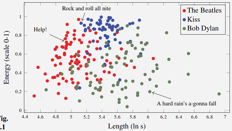
Figure 1 - Length vs Perceived Energy of Songs
- In this example, we want to classify the energy of a song based on it's length
- Note how the x axis of the graph is
- this is a common trick applied in machine learning for inputs that vary in size over several orders of magnitude.
- It is evident from the graph that in general:
- Kiss songs are more energetic
- Bob Dylan songs are longer
- Beatles songs are shorter
- However, the boundaries between these different classes are not clear.
- Therefore, oftentimes achieving 100% accuracy in machine learning is not possible.
- In this example, the length and energy features are not enough to precisely predict the song's energy
- We could add other features in the hope that there is some correlation between (some of) those features and the song's energy
Example - Car Stopping Distances
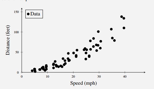
Figure 2 - Car Stopping Distances Example
- We now consider the car stopping distances dataset which contains 62 samples
- The dataset has two variables:
Speed: The speed of the car when the brake signal is givenDistance: The distance travelled after the signal is given, until the car has stopped
- We can clearly see that there is a trend in the data - the fastest the car, the longer the stopping distance
- We could create a model / function for this regression problem - given some speed, what is the expected stopping distance?
- Important to note that we don't care too much about the performance of the model on the training set
- What matters is the ability of the model to generalise to data that was not used for training
- One of the simplest models
- The output or prediction is determined by looking at the labels or true values of nearby points in the training set.
- This involves some sort of distance metric.
- Our data is as follows:
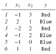
Figure 3 - Table of Values for KNN Classifier Example
- We can plot the data to visualise it as shown in Figure 4.
- To predict the output for some data-point
, we compute the distance from that data-point to every other data-point - We choose the
closest data-points, and take a majority vote (in the case of classification) or average (in the case of regression) to determine the output value - For
in the classification problem, we simply just choose the class of the closest neighbour - in this case has class red, so is red.
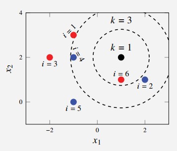
Figure 4 - KNN Classifier for k=1 and k=3
Data: Training data, denoted
Result: Predicted test output,
- Compute the distances
for all training points - Let
- Compute the prediction
using the following formula:
Is a parameter that must be chosen by the user - When
, the model is highly sensitive to local variations in the data - When
has a large value, it is less sensitive to local variations but can lose the ability to adapt to details in the data - boundaries are a bit smoother
- When
- We want to choose a value of
that is a compromise between the two - doesn't over-fit and doesn't under-fit.
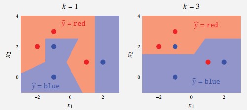
Figure 5 - KNN Decision Boundary for varying k-values
- We can also see the effect of changing
on the music dataset below:
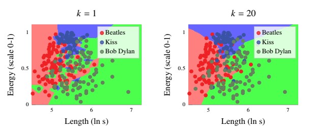
Figure 6 - KNN Decision Boundary for varying k-values
- We can apply the
-Nearest Neighbours technique to regression problem as well. - For each x-value, we compute the average of all data-points that exist within a range on the input axis.
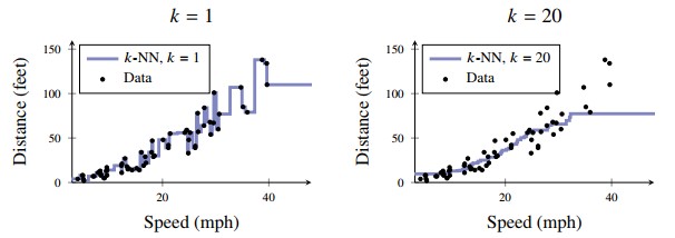
Figure 7 - KNN Regression Problem
Decision Trees
- Conceptually, applying a series of if-then rules to partition the input space.
- To make a prediction, start at the root of the try and apply the decision rule at each point to decide what branch to traverse down'
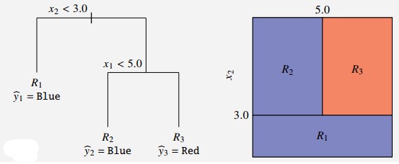
Figure 7 - KNN Regression Problem
Learning a Regression Tree
- The prediction
for a regression tree is a piecewise constant function of the input denoted
- Essentially, to learn a decision tree, we need to learn the threshold values at each level of the tree
- If our
values (input values) are continuous in nature, there are infinitely many sets of threshold values for our regression tree - However, the only time a prediction (on the training set) will change is when a threshold crosses a data point
- Even still, the search space is intractable
- The standard algorithm used to compute the regression tree is a greedy algorithm
- To get the predicted value for regression, we take the average of the training data-points that fall into a given region
Recursive Binary Splitting Algorithm
- At each split, we can only choose one of the
input variables - We split a given region
into two sub-regions denoted as:
- For each training data-point
, we can compute a prediction error by first determining which region the data-point falls in, and then computing the difference between and the constant prediction associated for that region - The computation for the SSE of all training points is denoted as:
- We want to minimise the difference between the predicted value and the actual value / ground truth
- For this reason, it makes sense to derive some sort of function that compares them
- This is precisely what the The Sum of Squared Errors (SSE) metric measures - low value if similar, high value if different.
- Using the SSE metric, the training problem is given as trying to minimise the SSE.
- To solve the machine learning problem using decision trees, we compute the split in between each of the values (all possible splits as shown by the dotted lines in the figure below) and compute its SSE
- We first compute the splits for the root node of the tree and choose the one with the lowest SSE
- Then "fix" that split and compute the splits for its children.
- Repeat until the depth of the tree reaches the desired limit
. - We can alternatively stop the algorithm's growth by setting a minimum number of data-points per leaf node (e.g., each leaf node must contain a minimum of 5 data-points.)
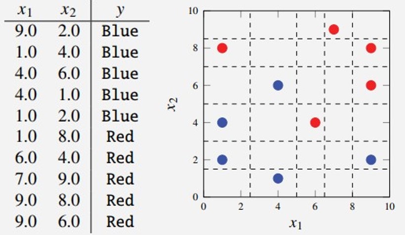
Figure 8 - Possible splits for decision tree problem
Regression Tree Algorithm
Goal: Learn a decision tree using recursive binary splitting:
Data: Training data
Result: Decision tree with regions
- Let
denote the whole input space - Compute the regions
- Compute the predictions
for as:
Function Split(R, 𝒯):
    if (stopping criterion fulfilled)
        return r
    else
        Go through all possible splits xⱼ < s for all input variables
          j = 1, ..., p
        Pick the pair (j,s) that minimises the loss function for regression/classification problems
        Split the region R into R₁ and R₂ according to Eq 2.4
        Split data 𝒯 into 𝒯₁ and 𝒯₂ respectively
        return Split(R₁, 𝒯₁), Split(R₂, 𝒯₂)
Classification Tree Algorithm
- This is very much the same for the application of the decision tree to the classification problem
- However, we must derive a new "loss function" for this categorical data
- Popular approaches include the misclassification rate, Gini index and entropy.
-
For example, we can construct a classification tree using the misclassification rate as our loss function
-
We introduce the following equation to denote the proportion of training observations in the
th region to belong to the th class - Note that in this equation
denotes the identity function, which returns 1 if and otherwise returns 0.
- Note that in this equation
-
We can then define the splitting criterion
based on these class proportions - Misclassification rate (proportion of data-points in region
which do not belong to the most common class) - Gini index:
- Entropy Criterion
- Misclassification rate (proportion of data-points in region
- Why are there these different classification algorithms?
- Introduce the concept of node purity
- A node is more pure if it assigns more of the same class to every data point that "comes its way"
- That is, nodes with higher purity can lead to fewer total splits in total
- The Gini Index and Entropy loss functions tend to be better than the misclassification rate.
- We can "stop training" a model by limiting the depth of the tree
- The effect of implementing this limit below for the classification problem
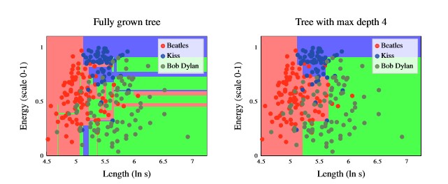
Figure 9 - Effect of varying depth of decision tree. Right Decision tree with unbound depth. We can see that the decision tree over-fits to the data.
- We can also show the effects on a regression problem
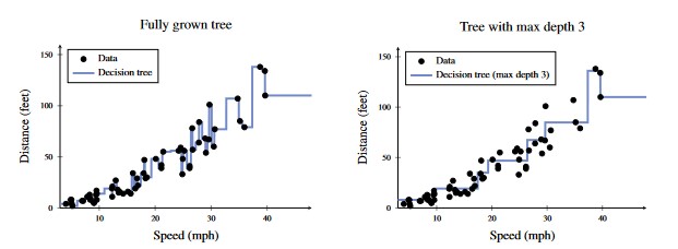
Figure 10 - Effect of varying depth of decision tree. Right Decision tree with unbound depth. We can see that the decision tree over-fits to the data.