COMP4702 Lecture 7

Neural Networks

A "neuron" in an (artificial) neural network is a highly simplified model of what goes on in a biological neuron
An artificial neuron is a processing unit that takes in several inputs via weighted connections.
The neuron computes a function of the sum of these weighted inputs and produces an output signal.

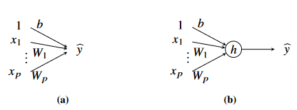
Figure 1 - Artificial Neuron (a) Generalised linear regression model (b) Output described as sum of all terms.

Observe that the illustration on the left describes the output $\hat{y}$ as the sum of all terms, $b$ and $\lbrace W_j x_j \rbrace _{j=1}^p$
- The generalised linear regression neuron (Figure 1 a) is the simplest type of neuron that we can have.
We can also have neurons that compute some other function $h()$ , which is a function of the weighted sum of the inputs.
- This is known as the activation function (an analogy to the idea of a biological neuron firing and producing an electrical output if it has enough stimulus in its inputs)
The two most common activation functions are the logistic sigmoid and the ReLU.

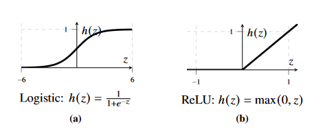
Figure 2 - Plots of two popular activation functions in Machine Learning - ReLU (Rectified Linear Unit) and the logistic (sigmoid) function

A linear neuron and a neuron with logistic activation are mathematically identical to the linear and logistic regression model.
A single layer of linear units can be trained to perform multiple linear regression (i.e. a regression model with multiple outputs)
A single layer of sigmoidal units is close to the multi-class regression model. Using softmax instead of logistic sigmoids will make it identical

Two-Layered Neural Network

If we have a single-layer model, then the notation $q_k$ is the output of the $k$ th neuron, $k=1, \cdots, U$ .

q_k = h(W_{k1} x_1 + W_{k2} x_2 + \cdots + W_{kp} x_p + b_k), \ \ \ \ \ k=1, \cdots, U \tag{6.4}

These outputs are connected to a second layer of neurons, which provide the final output of the model $\hat{y}$
- The first layer is called the hidden layer

\hat{y}=W_1 q_1 + W_2 q_2 + \cdots + W_U q_U + b \tag{6.5}

Every connection has a weight (parameter) so the notation $W_{7\ 3}^{(1)}$ denotes the weight from input 3 to neuron 7 in layer 1.

\begin{align*} q_1 &= h(W_{11}^{(1)} x_1 + W_{12}^{(1)} x_2 + \cdots W_{1\ p}^{(1)} + b_1^{(1)}),\\ q_2 &= h(W_{21}^{(1)} x_1 + W_{22}^{(1)} x_2 + \cdots W_{2\ p}^{(1)} + b_2^{(1)}),\\ \vdots\\ q_U&=h(W_{U1}^{(1)} x_1 + W_{U2}^{(1)} x_2 + \cdots W_{U\ p}^{(1)} + b_U^{(1)}),\\ \end{align*} \tag{6.6a}

Then out final model is denoted as

\hat{y}=W_1^{(2)}q_1 + W_2^{(2)}q_2 + \cdots + W_U^{(2)} + b^{(2)} \tag{6.6b}

There is also a bias/offset signal/weight for the hidden layer.

Vectorisation over Units

We observe that a two-layer (feed-forward) neural network (aka, multi-layer perceptron) can be written more compactly in terms of matrices and vectors.
The parameters in each layer are stacked in a weight matrix W, and an offset vector b

\begin{align*} {\bf{W}}^{(1)} &= \begin{bmatrix} W_{11}^{(1)} & \cdots & W_{1p}^{(1)}\\ \vdots & & \vdots \\ W_{U1}^{(1)} & \cdots & W_{U p}^{(1)}\\ \end{bmatrix}, \ \ \ \ &&{\bf{b}}^{(1)}= \begin{bmatrix} b_1^{(1)}\\ \vdots\\ b_U^{(1)} \end{bmatrix}, \\ W^{(2)} &= \begin{bmatrix} W_1^{(2)} & \cdots & W_U^{(2)} \end{bmatrix}, &&{\bf{b}}^{(2)} = \begin{bmatrix} b^{(2)} \end{bmatrix}, \end{align*} \tag{6.7}

Using this notation, the full model can then be written as:

\begin{align} &{\bf{q}} = h({\bf{W}}^{(1)} x + {\bf{b}}^{(1)}), \tag{6.8a} \\ &\hat{y}={\bf{W}}^{(2)} {\bf{q}} + {\bf{b}}^{(2)}, \tag{6.8b} \end{align}

The weight matrices and offset vectors are the parameters of the model, which can be compiled as a single vector (in the 2-layered perceptron shown above):

\def\vec{\text{vec}} \def\W {{\bf{W}}} \def\b {{\bf{b}}} \theta=\begin{bmatrix} \vec(\W^{(1)})^T & \vec(\b^{(1)})^T & \vec(\W^{(2)})^T & \vec(\b^{(2)})^T \end{bmatrix}

Deep Neural Networks

We can extend the model to any number of layers, creating a deep neural network
The notation $l \in \lbrace 1, \cdots, L \rbrace$ indexes the layers,and the number of units in the $l$ th layer is $U_l$ .
Each unit is fully connected to the inputs/units/output of the previous and next layer.

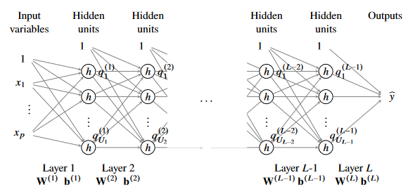
Figure 3 - An example of a deep neural network with L layers.

Observe that each layer of the neural network $l$ is parameterized by a weight matrix ${\bf{W}}^{(l)}$ and bias vector ${\bf{b}}^{(l)}$

In the early days of feed-forward neural networks, these models were seen as examples of parallel distributed processing.
If we think about an input signal propagating from the inputs through the layers, computation across units in any given layer is independent (and thus could be parallelised).
If we want to compute the output for a whole set of data points, computation required for each data point is independent.
Motivation to represent at vectors directly related to why GPUs are useful for deep learning.

Neural Networks for Classification

For the regression case, we just have linear activation on all the outputs.
For classification, we use the same building blocks.
For binary classification, a single output unit with logistic sigmoid can do the job
For $M>2$ classes, we have $M$ output units and use softmax ensuring that $\sum_{m=1}^M g_m=1$ where $g_m$ is the output value that estimates $p(y_i=m|{\bf{x}}_i)$ .
Example 6.1 demonstrates classification using neural networks on the MNIST dataset.

Example 6.1 - MNIST Problem

Figure 4 - Samples from the MNIST datasets

Dataset containing 28x28 pixel grayscale images of handwritten digits
Contains 60,000 training and 10,000 validation points
To feed the image into a Multi-Layer Perceptron, we flatten the 28x28=784 pixels into one long vector
Each item in the vector represents the intensity of the interval.
- After normalisation, the intensity value lies in the domain $[0,1]$ .
The will have to predict between 10 classes, representing each of the 10 digits.
Based on a set of training data $\lbrace{\bf{x}}_i, y_i\rbrace_{i=1}^{n}$ with images and labels, the problem is a good model for the class probabilities

p(y=m|{\bf{x}}), \ \ \ \ \ \ m=0, \cdots, 9

That is, the probability that some unseen image $\bf{x}$ belongs to each of the $M=10$ classes.
- Assume that we would like to use logistic regression to solve this problem with the softmax output
- This is identical to a neural network with just one layer.
- The parameters of this model would then be:

{\bf{W}}^{(1)} \in \mathbb{R}^{784 \times 10} \ \ \ \ \ {\bf{x}}^{(1)}\in \mathbb{R}^{10}

Which gives a total of $784\cdot 10 + 10 = 7850$ parameters.
Extending this model with a two-layer neural network with $U=200$ hidden units, that would require two sets of weight matrices and offset vectors:

\def\W{{\bf{W}}} \def\b{{\bf{b}}} \W^{(1)}\in\mathbb{R}^{782\times200}\ \ \ \ \b^{(1)}\in\mathbb{R}^{200},\ \ \ \ \W^{(2)}\in\mathbb{R}^{200\times10} \ \ \ \ \b^{(2)}\in\mathbb{R}^{10}

This produces a model with $784 \cdot 000 + 200 + 200 \cdot 10 + 10 = 159, 010$ parameters.

Training a Neural Network

Training is an optimisation problem over the parameters of the model.
If we want to refer to all of the model parameters, we collect all of the weights (and bias weights) and arrange them in a big vector $\theta$ .
The loss function is a sum over the losses for each data point in the training set.
Gradient descent is the basis of the most commonly used training algorithms
How can we get the gradient for a multi-layer neural network with non-linear activation functions?

Backpropagation

Lindholm uses "backpropagation" to refer to computing the gradient
To get the gradient for MLPs, calculus chain rule is critical.
Mathematical expressions in book can be interpreted as follows:
Need partial derivative of $J(\theta)$ with respect to each weight (and bias weight), in each layer of the network (Eq 6.22).
- The gradients with respect to the weights are given as:
  $\def\W{{\bf{W}}} dW^{(t)} \overset{\triangle}{=} \nabla_{\partial\W^{(l)}} J(\theta) = \begin{bmatrix} \frac{\partial J(\theta)}{\partial\W_{11}^{(l)}} & \cdots & \frac{\partial J(\theta)}{\partial\W_{1,U^{(l-1)}}^{(l)}}\\ \vdots && \vdots \\ \frac{\partial J(\theta)}{\partial \W_{U^{(l)},1}^{(1)}}& \cdots & \frac{\partial J(\theta)}{\partial \W_{U^{(l)},U^{(l-1)}}} \end{bmatrix} \tag{6.22a}$

d{\bf{b}}^{(l)} \overset{\triangle}{=} \nabla_{\partial {\bf{b}}^(l)} J(\theta)=\begin{bmatrix} \frac{\partial J(\theta){\partial b_1}}{\partial b_1^{(l)}}\\ \vdots\\ \frac{\partial J(\theta){\partial b_1}}{\partial b_{U^{(l)}}^{(l)}}\\ \end{bmatrix}

We use these to do our update for gradient descent (Eqn 6.23)

\def\W{{\bf{W}}} \def\b{{\bf{b}}} W_{t+1}^{(l)} \leftarrow \W_t^{(l)} - \gamma d\W_t^{(l)},\tag{6.23a}

\def\W{{\bf{W}}} \def\b{{\bf{b}}} b_{t+1}^{(l)} \leftarrow \b_t^{(l)} - \gamma d\b_t^{(l)},\tag{6.23b}

Derivation of Backpropagation

The backpropagation step of a network consists of two steps - forward propagation and backpropagation

Forward-Propagation

In the forward propagation step, the cost function is evaluated using the neural network model.
We start with the input $\bf{x}$ which is an input to the first layer.

{\bf{q}}^{(0)}={\bf{x}}\tag{2.64a}

We repeatedly apply the weight and bias to the previous layer's output.
- $\bf{z}^{(l)}$ is the weighted sum of inputs before the application of the activation function $h$ .
- $\bf{q}^{(l)}$ is the output of the perception

\begin{cases} {\bf{z}}^{(l)} = {\bf W} ^ {(l)} {\bf q} ^ {(l-1)} + {\bf b}^{(l)}\\ q^{(l)} = h({\bf{z}})^{(l)} \end{cases} \text{for} l=1, \cdots, L-1 \tag{6.24b}

We the evaluate the last layer, $L$ .

{\bf{z}}^{(L)}={\bf{W}}^{(L)} {\bf{q}}^{(L-1)} + {\bf{b}}^{(L)} \tag{6.24c}

Given the output of the model, denoted ${\bf{z}}^{(L)}$ , we compute the cost function of the model to evaluate the performance of the model.

J(\theta) = \begin{cases} (y-z^{(L)})^2, &\text{if regression problem,}\\ -z_y^{(L)} + \ln\sum_{j=1}^M e^{z_j^{(L)}}, &\text{if classification problem} \end{cases} \tag{6.24d}

Observe that the objective function uses the squared difference for regression, and cross-entropy for classification.

Back-Propagation

The gradient with respect to the (total weighted sum of) input signals to the units in a layer $d{\bf{z}}^{(l)}$ and the output signals of units in a layer $d{\bf{q}}^{(l)}$ given in Eq 6.25
$d{\bf z}\triangleq \nabla_{z^{(l)}} J(\theta) = \begin{bmatrix} \frac{\partial J(\theta)}{\partial z_1^{(l)}}\\ \vdots\\ \frac{\partial J(\theta)}{\partial z_{U^{(l)}}^(l)} \end{bmatrix} \tag{6.25a}$

d{\bf q}^{(l)} \triangleq \nabla_{{\bf{q}}^{(l)}} J(\theta)= \begin{bmatrix} \frac{\partial J(\theta)}{\partial q_1^{(l)}}\\ \vdots\\ \frac{\partial J(\theta)}{\partial q_{U^{(l)}}^{(l)}} \end{bmatrix} \tag{6.25b}

Then, we start calculating the gradients at the output layer, using the derivative of the activation function and $J$ in Eq 6.26.
- 6.26a describes that for regression problems, the derivative at the end of our MLP which uses squared-error loss is given by:
  
  $dz^{(L)} = \frac{\partial J(\theta)}{\partial z^{(L)}} (y-z^{(L)})^2 = -2 (y-z^{(L)}) \tag{6.26a}$
- 6.26b describes the derivative for a multi-class classification problem with cross-entropy loss.
  $dz_j^{(L)} = \frac{\partial J(\theta)}{\partial z^{(L)}} = \frac{\partial}{\partial z^{(l)}}(-z_y^{(L)} + \ln \sum_{k=1}^{M} e^{z_k^{(L)}}) = - \mathbb{I}\lbrace y = j \rbrace + \frac{e^{z_j^{(L)}}}{\sum_{k=1}^{M} e^{z_k^{(L)}}}$
The gradients for the weight and bias weights in that layer can be computed, and the gradient signals in the current layer are used to compute the gradients for the previous layer Eq 6.27

d{\bf{z}}^{(l)} = d{\bf q}^{(l)} \odot h' ({\bf z}^{(l)}) \tag{6.27a}

d{\bf{q}}^{(t-1)} = {\bf W}^{(t)T} d({\bf z}^{(l)}) \tag{6.27a}

Note here that $\odot$ denotes the element-wise product and $h'(z)$ is the derivative of the activation function $h(z)$ .
- $h'({\bf{z}})$ acts element-wise on $\bf z$

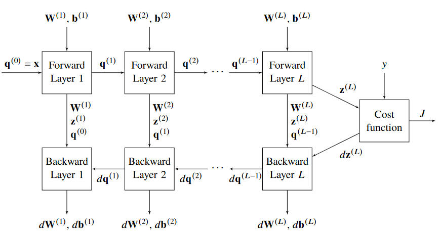
Figure 5 - Graphical representation of the backpropagation algorithm

Observe that in each of the forward propagation steps, the weights, weighted sum and neuron output are recorded to be used later.
Furthermore, in the backpropagation step, we need the gradient with respect to the weight matrix and bias vector.
All equations used for backpropagation can be derived from the chain rule of calculus.
So far, we have only considered backpropagation for one data point.
- However, we do want to compute the cost function $J(\theta)$ and its gradients $d {\bf{W}}^{(t)}$ and $d{\bf{b}}^{(t)}$ for the whole mini-batch $\lbrace {\bf{x}}_i, y_i \rbrace_{i=(j-1) n_b+1}^{jn_b}$ .
Therefore, run Eq. 6.24, 6.26 and 6.27 for all data points in the current mini-batch and average their results for $J$ , $d{\bf W}^{(l)}$ and $d{\bf b}^{(l)}$ ,
To do this in a computationally efficient manner, process all $n_b$ data points in the mini-batch simultaneously by stacking them in matrices where each row represents one data point

Backpropagation - Algorithm

Input:

Parameters ${\bf{\theta}} = \lbrace {\bf{W}}^{(l)}, {\bf{b}}^{(l)}\rbrace_{l=1}^{L}$
Activation function $h$
Data $\bf{X}, y$ with $n_b$ rows where each row corresponds to one data point in the current mini-batch Result: $J(\theta)$ , $\nabla_\theta J(\theta)$ of the current mini-batch

Forward-Propagation
Set ${\bf{Q}}^0\leftarrow \bf{X}$
for $l=1,\cdots, L$ do
| ${\bf{Z}}^{(l)} = {\bf{Q}}^{(l)T} + {\bf{b}}^{(l)T}$
| ${\bf{Q}}^{(l)} = h({\bf{Z}}^{(l)})$ Do not execute this line for the last layer $l=L$
end
Evaluate the cost function
if Regression problem then
| $J(\theta)=\frac{1}{n_b} \sum_{i=1}^{n_b} (y_i-Z_i^{(L)})^2$
| $d{\bf{Z}^{(L)}}=-2({\bf{y}}-{\bf{Z}}^{(L)})$
else if Classification problem then
| $J(\theta) = \frac{1}{n_b} \sum_{i=1}^{n_b} (-Z_{i,y_i}^{(L)} + \ln (\sum_{j=1}^{M} \exp (Z_{ij}^{(L)})))$
| $dZ_{ij}^{L}=-\mathbb{I}\lbrace y_i=j\rbrace + \frac{\exp (Z_{ij}^{(L)})}{\sum_{j=1}^M \exp(Z_{ij}^{(L)})} \ \ \ \ \forall i,j$
Backward Propagation
for $l=L,\cdots,1$ do
| $d{\bf Z}^{(l)}=d{\bf{Q}}^{(l)}\odot h' ({\bf{Z}}^{(l)})$ Do not execute this line for the last layer $l=L$
| $d{\bf Q}^{(l-1)} = d{\bf{Z}}^{(l)}{\bf{W}}^{(l)}$
| $d{\bf W}^{(l)} = \frac{1}{n_b} d{\bf{Z}}^{(l)T}{\bf{Q}}^{(l-1)}$
| $d{\bf b}^{(l)}_j = \frac{1}{n_b} \sum_{i=1}^{n_b} dZ_{ij}^{(l)}\ \ \ \ \ \ \forall j$
end
$\nabla_\theta J(\theta)=\begin{bmatrix}\text{vec}(d{\bf{W}}^{(1)})^T & d{\bf b}^{(1)T} & \cdots & \text{vec}(d{\bf W}^{(L)})^T & d{\bf b}^{(L)T}\end{bmatrix}$
return $J(\theta), \nabla_\theta J(\theta)$

Weight Initialisation

Weights are typically initialised to small, random values at the start of gradient-descent based training

MNIST Classification

We see the effect of a single-layered logistic regression model vs one with a single hidden layer.

Use Stochastic Gradient Descent with $\gamma=0.5$ and mini-batch $n_b=100$
- Since there are 60,000 training points in total, one epoch is completed after $60\ 000 / 100 = 600$ iterations
- Run the algorithms for 15 epochs

Figure 8 - Effect of adding an additional layer to the MNIST classification example.

In the original model, the misclassification rate is approximately 8% on validation data
The addition of a new hidden layer with $U=200$ hidden units and ReLU activation function is given.
- It decreases the misclassification rate to 2%

Convolutional Neural Networks

Big part of the reason why deep learning has been a popular part of the surge of interest in AI/ML.
Fundamental idea to take into account structure in data, specifically in terms of relationship between different inputs in the data
CNNs were originally applied to image data, but have been applied to other types of data with spatial and/or temporal structure

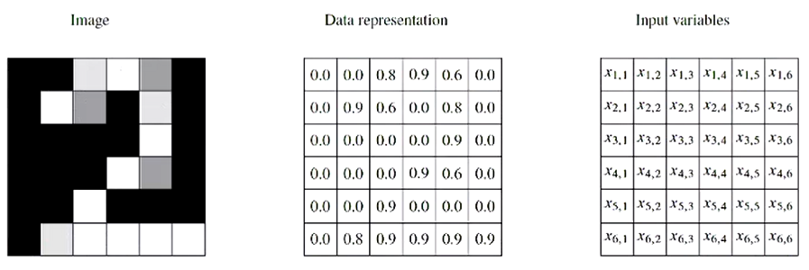
Figure 9 - The process of converting an image (e.g. sample like MNIST) into matrix representation

When converting an image into the data representation, we convert the image into its data representation, in which the number represents the intensity of the pixels.
The pixel values are stored in a matrix with elements denoted $x_{j,k}$ .
If we have 36 hidden units for this output, a fully connected (dense) layer would require 1296 weights (plus biases).
Convolutional layers have far fewer parameters and do so by enforcing some useful structure:
- Sparse Interactions: Lining up the input matrix with the hidden matrix, only a limited local region of inputs are connected to each hidden unit, in which the borders are typically handled with zero-padding.
- Parameter Sharing: Rather than having separate weights for each hidden unit, force all hidden units to have the same weight values, called a "filter".
  - The weights in the filter are learned in every position that the filter can be in
  - Can have more than one filter in a layer, with each filter having its own weight parameters
The convolution operation is mathematically represented with the following equation:

q_{ij}=h\left(\sum_{k=1}^{F} \sum_{l=1}^{F} x_{i+k-1,j+l-1} W_{k,l}\right) \tag{6.29}

In this equation, $x_{i,j}$ denotes the zero-padded input to the layer
- $q_{ij}$ output of layer
- $W_{k,l}$ Filter with $F$ rows and $F$ columns

Figure 9 - An example of how the convolution of a matrix is computed. Each hidden unit's value is only dependent on a small region of pixels around its location

This can be thought of as the same as the fully-connected/dense network where each of the weights that are not in the neighbourhood are set to 0.
The properties of Sparse Interactions and Parameter Sharing make the CNN relatively invariant to translations of objects in images

Strides in Convolutional Neural Networks

Another technique to reduce computation is to move the filter (input window) by more than one pixel at a time when computing the output as shown in the figure below.
Thinking about the hidden units as activation values obtained by moving the filter around
The number of hidden units is determined by the filter size and stride.
The edges can get messy depending on what sizes are chosen.

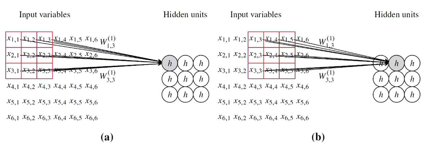
Figure 10 - An example of how the convolution of a matrix is computed. Each hidden unit's value is only dependent on a small region of pixels around its location

Pooling Layer in Convolutional Neural Network

A layer that has no trainable parameters, but used as a component to reduce the size of the model
Done by computing average / maximum of values over a given filter size.
- In the first iteration of the figure, $\max(5,2,2,3)=5$
- In the second iteration of the figure $\max(1,0,0,3)=3$

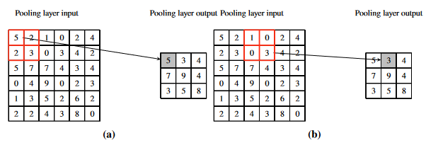
Figure 10 - An example of how the convolution of a matrix is computed. Each hidden unit's value is only dependent on a small region of pixels around its location

Pooling can make the model more invariant to (small) translations of the input

Multiple Convolutional Channels

With a single filter, we produce a matrix of "hidden units"
If we use multiple filters, we get a stack of these matrices called channels.
The hidden layer of units is a tensor $(\text{rows} \times \text{columns}\times\text{channels})$
When a CNN is trained on colour images, it is typical to have one (or more) separate channels for the Red, Green and Blue intensity values of each pixel in the image.

Full CNN Architecture

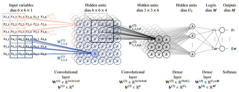
Figure 11 - An example architecture for a convolutional neural network used for the classification of 6x6 grayscale images

The typical CNN architecture is shown above.
Typically have a series of convolutional layers to decrease the dimensionality of the images
Then have some dense layers (a MLP) to take the convolution outputs and classify them
In the case of classification, the last layer has $N$ outputs - one for each class.
- The output is encoded in the one-hot fashion.

Dropout

When training, randomly set some hidden units to 0 so that they don't do anything.
Compute the gradient for the remaining sub-network
On the next training iteration, choose other layers to drop out
This can reduce model complexity.
Finally at the end of training all the hidden units are restored and used together.