COMP4702 Lecture 9

Chapter 8: Non-Linear Input Transformations and Kernels

Creating Features by Non-Linear Input Transformations

What if we perform some non-linear transformations of the data before passing to the model?

The vanilla linear regression model is denoted as:

From this, we can extend the model with $x^2, x^3, \dots, x^{d-1}$ as inputs in which $d$ is another hyperparameter, we can obtain the following model:

Since $x$ is know, we can directly compute the exponents $x^2, x^3, \dots, x^{d-1}$. Note that this is still a linear regression model since the parameters $\theta$ appear in a linear fashion with ${\bf{\phi}}(x)=\begin{bmatrix}1&x&x^2&\cdots&x^{d-1}\end{bmatrix}^T$ as a new input vector, a vector of basis functions

• One of these transformations of $x$ is known as a feature, and the vector of transformed inputs is denoted ${\bf{\phi}}(x)$.

% Create our dataset
x = rand(20,1);
y = cos(x)
% Add some noise 
y = y + 0.1*randn(20,1);

x1 = linspace(0,1)
y1 = polyval(p1, x1);
hold on;
plot(x1,y1);
xsqd = x.^2;
xcub = x.^3;
z = [x xsqd xcub];

% Now do polynomial fitting on z
b = ones(20,1); % Bias vector
z = [b z];
% Training step, p3 are our theta values
p3 = inv(z'*z)*z'*y;

% Create test set
y3 = zeros(1,100);
for i=1:100
y3(i) = p3(1) + p3(2)*x1(i) + p3(3)*x1(i.^2) + p3(4)*x1(i.^3);
end
plot(x1,y3);

Kernel Ridge Regression

• The most important idea in this chapter is the use of a kernel function $\kappa({\bf x}, {\bf x}')$ between two datapoints ${\bf x}$ and ${\bf x}'$.

• If we have a set of non-linear basis functions ${\bf \phi}({\bf x})$ then a very useful kernel function is the inner product between these pairs of datapoints:

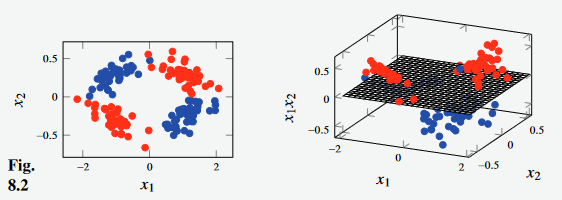
• From the example below, it is evident why adding the polynomial inputs allow models to achieve superior performance.

  • With the input space to the left, the red and blue datapoints are not distinguishable by a linear model.
  • However, by introducing $x_1 x_2$ as a third input feature, the data becomes (almost perfectly) linearly separable by a single plane.

• We can expression linear regression with MSE and $L^2$ regularisation as follows, replacing $x$ with $\phi(x)$ as we want to ues the basis function transformation of each input variable.

• We can re-write this equation as inner products of basis functions, yielding Equation 8.7 shown below.

• For a training set $\bf X$, the matrix ${\bf\Kappa}({\bf X}, {\bf X})$ is the kernel function applied to all pairs of data points.

  • ${\bf\Kappa}({\bf{X, x_\star}})$ is a vector where we calculate the kernel function between a test point $\bf{x_\star}$ and all points in the training set.

  • This brings us to kernel ridge regression, where the predictions are given by Equation 8.14b using $\hat\alpha$ Equation 8.14a and the kernel function across the training set ${\bf X}$ and the test point ${\bf x_\star}$ denoted as $\Kappa({\bf X, x_\star})$.

    $$\hat\alpha=\begin{bmatrix}\hat\alpha_1\\\hat\alpha_2\\\vdots\\\hat\alpha_n\end{bmatrix}={\bf y^T} ({\bf \Kappa} ({\bf X,X}) + n\lambda {\bf I})^-1 \tag{8.14a}$$
    $$\hat{y}({\bf x_\star}) = \hat\alpha {\bf \Kappa} ({\bf X,x_\star})\tag{8.14b}$$

  • Instead of computing a $d$-dimensional vector $\hat\theta$, we compute and store a $n$-dimensional vector $\hat\alpha$ (from Equation 8.14a) as well as ${\bf X}$.

• Require that the kernel is positive definite - these kernels are known as positive semidefinite kernels
  • This comes from the requirement that ${\bf \Kappa}({\bf X, X}) + n \lambda {\bf I}$ has an inverse.
• One potential choice of the kernel function is the Squared Exponential Kernel / Gaussian kernel:

• In Equation 8.13 above, $\ell>0$ is a hyperparameter that is left to be chosen by the user.
• Kernel Ridge regression predicts based on the value of the kernel function between the test point and all training points weighted by the $\hat\alpha$ terms from Equation 8.14a.
• We can see that when we get $\hat\alpha$ by adding "a bit of" identity matrix to $\bf\Kappa({\bf X,X})$ and inverting that and multiplying by the target values from the training set, ${\bf{y}}^T$, we are essentially adding a bit of noise to the diagonal of the kernel matrix.

• How does this work?
  • Start by writing down the loss function, and its solution, the prediction function for linear regression (with $L^2$ regularisation) in terms of the transformed data ${\bf\phi}({\bf x})$ in place of $\bf x$
    • We can do this as linear regression has a closed-form solution
  • Use some matrix algebra to realise that we can re-write the solution in such a way that ${\bf\phi}({\bf x})$ only appears as inner products ${\bf\phi}({\bf x})^T {\bf\phi}({\bf x}')$.
  • That gives our kernel function. We can use the kernel function and we will be using the same model, loss function and prediction function
• Note that when we write linear regression in the previous form (Equation 8.5),we have a $d$-dimensional parameter vector $\theta$ no matter how big $n$ is (the size of the training set)
• Now, we compute the kernel function for all pairs of datapoints, so the size of our "model" is in terms of $n$ not $d$.
• We can use kernels that allow $d\rightarrow\infty$.

Matlab Example

% Create our dataset
x = 5 * rand(50,1);
y = x.^2 + 2*randn(50,1); % Our function is y = x^2 (+ noise)

plot(x,y,'.');
% Number of training points
n = 50;           
% Hyperparameter, weight of regularisation in loss function
lambda = 0.01;    
% Kernel function hyperparameter
l = 5;            
d = pdist(x); % Euclidean distance between datapoints
% Evaluate kernel function
k = exp(-(d.^2)/(2*l^2));
K = squareform(k); % Turn into square matrix
alpha = (y'*inv(K + n*lambda*eye(n,n)));
% Prediction
xtest = 0:0.1:5;
dtest = pdist2(xtest',x);
ktest = exp(-(dtest.^2)/(2*l^2));
ytest = ktest*alpha;
hold on;
plot(xtest,ytest,'k');

Support Vector Regression

• Support Vector Regression means changing the loss function from that used in kernel ridge regression to the $\epsilon$-insensitive loss (Equation 8.17).

  $$\begin{align*} L(y,\hat y)&= \begin{cases} 0, &\text{if } |y-\hat y|\lt\epsilon\\ |y-\hat y|-\epsilon, &\text{otherwise}, \end{cases} \tag{8.17}\\ &=\max(0, |y-\hat y| - \epsilon) \end{align*}$$
  • This no longer has a closed-form solution, so we require a numerical optimiser to solve.
  • However, the problem is a convex, constrained optimisation problem so there are likely fewer issues than with neural network training
  • Optimising this loss function leads to many of the $\alpha_i$ values becoming exactly zero.
    • This means that in the end, the trained model only depends on a small number of the data points to make its predictions

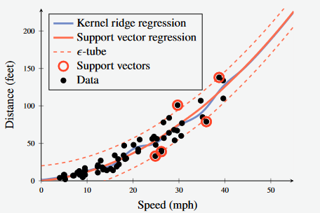
• All datapoints inside the dashed lines don't affect the prediction
  • The datapoints outside are known as the support vectors, and affect the prediction

Kernel Theory

• It turns out that several ML models can be re-written as kernel methods.
• We can do this for k-NN, by writing the (squared) Euclidean Distance in terms of a linear kernel:
  $$\kappa ({\bf x,x}')={\bf x}^T {\bf x}'$$

• One of the main reasons that kernel methods became widely used in Machine Learning is that they allow you to apply ML techniques to data where Euclidean Distance cannot be defined (e.g. text snippets, in Example 8.4)
  • They effectively allow you to "make up" your own kernel method.
  • If you can create a sensible way to compare datapoints, then you can use kernel methods

Example 8.4 - Kernel k-NN for Interpreting Words using Levenshtein Distance (Edit Distance)

• With textual inputs, Euclidean distance has no meaning.
• We can use the Levenshtein Distance (Edit Distance) to compare two strings.
  • This is the number of single-character edits required to transform one word (string) to the other.
• LD returns a non-negative integer which is only zero if the two strings are equivalent.
  • This fulfils the properties of being a metric on the space of character strings.
• Using LD, we can construct the kernel as:

• Consider a training set with 10 adjectives ($x_i$) and corresponding labels $y_i \in \lbrace\text{Positive, Negative}\rbrace$ according to their meaning.
• Use a kernel $k-NN$ with the kernel defined above to predict whether the word $x_\star=$'horrendous' is a positive or negative adjective.

• Inspecting the rightmost column, the closest word to horrendous is 'tremendous'.
  • Thus, if we use $k=1$, the conclusion would be that 'horrific' is a positive word.
• However, the third, second, fourth closest words are all negative (dreadful, horrific, outrageous).
  • Thus, if we use $k=3,k=4$, the conclusion would be that 'horrific' is a negative word

Meaning of a Kernel

• There is a lot of freedom in choice of a Kernel Function.
  • Many kernel functions that are commonly used are positive semidefinite, but for practical purposes, this doesn't mater (Except for kernel ridge regression)
  • A number of example functions are discussed in the book.

• The kernel defines how close (or similar) any two data points are.
  • if $\def\x{{\bf x}}\kappa(\x_i, \x_\star) > \kappa (\x_j, x_\star)$ then ${\bf x}_\star$ is more similar to ${\bf x}_i$ than ${\bf x}_j$.
  • For most methods, the prediction $\hat y ({\bf {x}}_\star)$ is most influenced by the training points that are closest or most similar to ${\bf x}_\star$
• Even though we started by introducing kernels via the inner product ${\bf\phi}({\bf x})^T{\bf\phi}({\bf x}')$, we do not have to bother about the inner product for the space itself in which $\bf x$ lives.
  • We can also apply a positive semi-definite kernel method to text strings without worrying about the inner product of strings, as long as we have a kernel for that type of data.

Valid Kernels

• There are many examples of kernels, and the book goes into detail regarding what constitutes a valid kernel.
• Examples of kernels include the linear kernel (Equation 8.23) and the polynomial kernel (Equation 8.24) in which the order of the polynomial is $d-1$

Support Vector Classification

• We can reason about Support Vector Classification using the same argument with logistic regression (as we did for linear regression + Support Vector Regression)

• If we use the hinge loss function for logistic regression (with transformed inputs; output of basis function), we end up with a training problem that is convex-constrained optimisation problem (which requires a numerical solver)

  • When this is solved, the solution again tends to be sparse (many $\alpha_i=0$).

• When the margin for a datapoint is $>1$, then $\alpha_i=0$ so in the end these datapoints don't define the decision boundary.

• When the margin for the data point $i$ is $<=1$ the point is inside the margin or on the wrong side of the decision boundary.

• The classification model is given as:

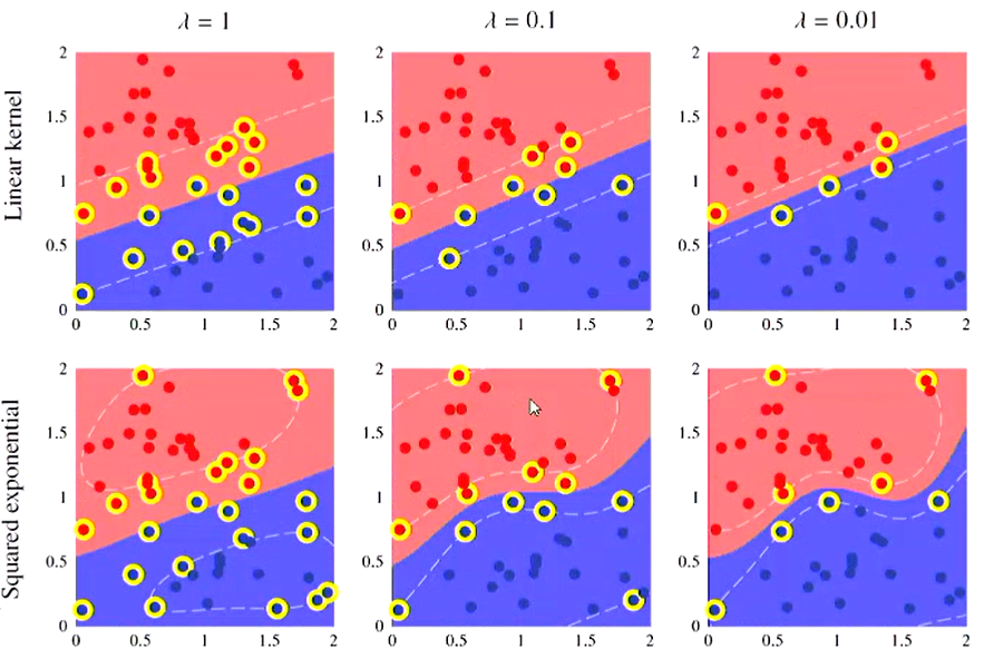
• Note that $\lambda>0$ is a regularisation parameter that penalises points that are inside the margin.
• Im ML libraries, you will often find this parameter as $C=\frac{1}{\lambda}$ or possibly even $\nu$
• The effect of this can be seen in the horizontal of Figure 3 above.