Deep Generative Models

Invertible non-Gaussian Models and Normalising Flows

Optional reading

Generative Adversarial Networks

• Consider the task of modelling a complex, high-dimensional probability distribution $p({\bf x})$.
• The approach here is to build a ML model (e.g., Deep Neural Network) that can transform a data point $\bf z$ into $\bf x$.
  • If $\bf z$ corresponds to a sample from a simple distribution like a Gaussian distribution, the network could then be used to transform this sample into a sample from the complex probability distribution $p({\bf x} | {\bf \theta})$.
  • We could then use this approach to generate new data for some interesting problems such as images
  • How can we learn such a network from data?

• The basic idea of Generative Adversarial Networks (GANs) is to compare the training data with synthetic samples generated from the model.
• If we can iteratively modify the model so that synthetic samples become more and more similar to the training data, we get closer to our goal.
• This is done via steps of a "game": (Lindholm et al, Page 273)
  1. Flip a coin (set $y=1$ with probability $0.5$ and $y=-1$ with probability $0.5$)
     1. If $y=1$ then generate a synthetic sample from the model ${\bf x}'\sim p({\bf x} | {\bf \theta})$. That is, sample ${\bf z}'\sim\mathcal{N}(0,I)$ and compute ${\bf x}'=f_\theta({\bf z}')$.
     2. If $y=-1$ then pick a random sample from the training data instead. That is, we set ${\bf x}'={\bf x}_i$ for some index $i$ sampled uniformly at random from $\lbrace 1, \cdots, n\rbrace$.
  2. Ask a critic to determine if the sample is real or fake. For instance, in the example with pictures of faces, we could ask the question "Does ${\bf x}'$ look like a real face or is it synthetically generated?"
  3. Use the critic's reply as a signal for updating the model parameters $\theta$. Specifically, update the parameters with the goal of making the critic as 'confused as possible' (maximise the loss function), regarding or not whether the sample presented is real or fake.
• We need a critic, whose job is to determine whether or not a data point is real or synthetic. The learning in the generative model then aims to try to confuse the critic.
• The critic is a classifier, which takes as input a datapoint and predicts the probability that it is synthetic.
  • The labels come from the gale above, nad the critic is trained to minimise the loss function, given in Equation 10.26 below.
    $$\hat{\bf\eta}=\arg\min_\eta \mathbb{E} \left[L(y, g_\eta({\bf x}'))\right]\tag{10.26}$$
  • From the perspective of the critic, it is attempting to minimise the loss denoted $\eta$
    $$\min_\eta \lbrace \frac12 \mathbb{E} \left[L(1, g_\eta(f_\theta({\bf z}')))\right] + \frac12\mathbb{E}\left[L(-1,g_\eta({\bf x}_i))\right]\rbrace\tag{10.27}$$
  • The objective of the generative model as a whole is to maximise the classification loss of the critic (Equation 10.27) with respect to $\theta$
    $$\max_\theta \min_\eta \lbrace \frac12\mathbb{E}\left[L(1,g_\eta(f_\theta({\bf z}')))\right] + \frac12 \mathbb{E}\left[L(-1, g_\eta({\bf x}_i))\right]\rbrace\tag{10.28}$$
• This results in a minimax problem, where two adversaries (critic, generative model) compete for the same objective, one trying to minimise it and the other trying to maximise it.
  • Typically the problem is approached by alternating between updating $\theta$ and updating $\eta$ using stochastic gradient optimisation.

Representational Learning and Dimensionality Reduction

• Consider SciKit Learn's Swiss Roll dataset, which has been plotted below:

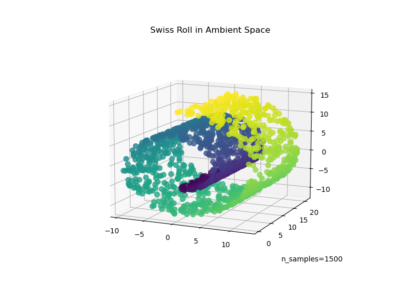
• Attempting to predict the value of the data points with traditional linear regression would be quite difficult given the high dimensionality of the data.
• However, this is actually quite a simple shape - it's a 2D manifold embedded in 3D space.
  • This manifold has a linear gradient of colour (color corresponding to the value)
  • If we could "unroll" the data, linear regression would get very high accuracy.
• Dimensionality reduction in ML is all about trying to learn a useful representation of high-dimensional data.
• A nice way to think about this is learning the structure among the columns (features) of a dataset, rather than clustering which learns about structure among the rows (data points).

Auto Encoder

The neural network solution to reducing dimensionality.

• An Autoencoder is a neural network that can be trained to perform dimensionality reduction, from unsupervised data, using a supervised learning algorithm
• We can see from the structure that the network tries to learn an identity mapping, so that the target output for some input vector is the input itself (the model's desired output is the input).
• The hidden layer is the bottleneck, and the network is trained to learn a compressed representation of the input data.
• This would be trivial, except that the hidden layers of the network have different numbers of units - typically fewer units than the number of inputs
  • This creates a bottleneck within the network
• For the network to perform well, it has to learn a good internal/latent representation of the data in a space of lower dimensionality.

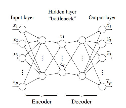
• Autoencoders typically have this symmetrical structure and can be trained with backpropagation / gradient descent.
  • The first half of the network is called the encoder and the second half the decoder.
• The decoder can be used as a generative model, and this idea has been used to develop several popular techniques in deep generative models.
• The encoder component can be used to translate an input of dimensionality $1\times p$ to dimensionality $1\times q$.
• Conversely, the decoder component can be used to translate an input of dimensionality $1\times q$ to dimensionality $1\times p$.

Principal Component Analysis (PCA)

• PCA can be thought of as performing a rotation of the coordinate system of the data space, to align the coordinate axes with the directions of greatest variance in the data.
• Dimensionality reduction can then be done by projecting the data onto a subspace of the new coordinate system.
• The solution of PCA gives us the basis vectors of the new coordinate system, together with a measure of the amount of variance (aka the principal values) that is captured by each of the basis vectors (aka the principal components).
• To use PCA, you need to mean-center the data for each variable.

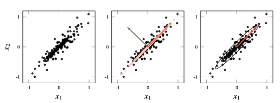
• In the left plot, we see some data in 2D space.
• The middle plot shows the first (red) and second (green) principal axes - these vectors are given by the first and second vectors of $\bf V$
  • The plot also shows datapoints when projected onto the first principal axis (pink) - this step reduces the dimensionality of the data from 2D to 1D.
  • You can express the values along this principle component as a linear combination of $x_1, x_2$
• The third plot shows an ellipse fitted to the covariance matrix $\frac 1n {\bf X}_0^T {\bf X}_0$ of the data.

• Lindholm et al covers PCA using Singular Value Decomposition (SVD) which is the mot efficient way.

• A simpler and more intuitive way is to compute to covariance matrix and then find its eigenvectors and eigenvalues

• In both cases, a closed-form solution exists and no iterative optimisation is required.

• From PCA, you can generate a scree graph which demonstrates how much each principal component (horizontal axis) contributes toward the variance.

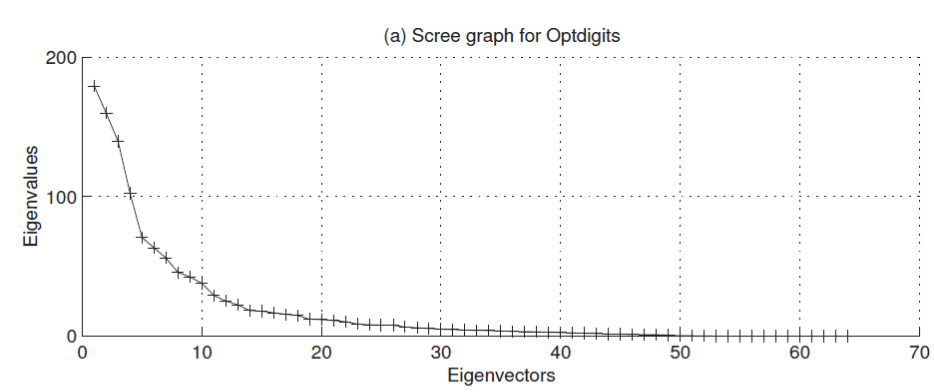
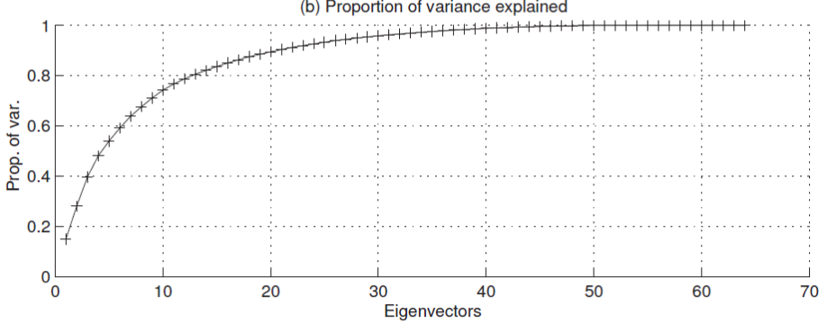
• Figure 4 above demonstrates that if we reduce the dimensionality of the data from the original 64 down to 10, we will still capture $\approx 75$ of the variance in the data.
• Reducing the dimensionality to 2 or 3 dimensions can be used to visualise data with an appropriate amount of dimensionality.

User Aspects of Machine Learning

Not assessable.

This chapter gives some general practical advice about the application (engineering) of machine learning. It's a mostly non-technical read and it is very useful stuff, but we will be fairly brief in covering it. The key points include:

• It is important to handle data carefully (training/validation/test splits), unintended relationships in datasets, variations over collection/observation time, etc.
  • Make sure to shuffle your data before splitting.
• Trying to summarize performance in a single number is at best a huge loss of information (cf. compression).
• Establishing baselines and bounding possible performance is incredibly important (but often not done).
• Try simple things first (Occam's razor).
• Debugging can be tricky.
• Training error/generalisation gap stuff (recall Chap.4)
• Error Analysis (this is a great subsection!): evaluating an ML model should not be just calculating an accuracy rate. We should look at which data points it is getting incorrect. Is it something about the data (e.g. lighting in images)? In a real world application, working with a domain expert, this would be an iterative, interactive process.
• Getting more data is always good, but if we can't: maybe add some slightly different data; data augmentation; transfer learning; learning from unlabelled data.
• Outliers are somehow unusual and they might be useless (e.g. noise, incorrect measurement), but they could also be important to the problem. Generic outlier removal is a dangerous thing to do: you are changing the distribution of the data in an unprincipled way.
• Missing data: discarding rows, imputation.
• Feature selection: connection to L1 regularisation, correlations, PCA.
• Can I trust my ML model? Understanding why a prediction was made, transparency.
• Worst case guarantees: individual bad predictions for a class, etc.